Spatial Dynamics of Invasive Para Grass on a Monsoonal Floodplain, Kakadu National Park, Northern Australia


Abstract
:
1. Introduction
2. Materials and Methods
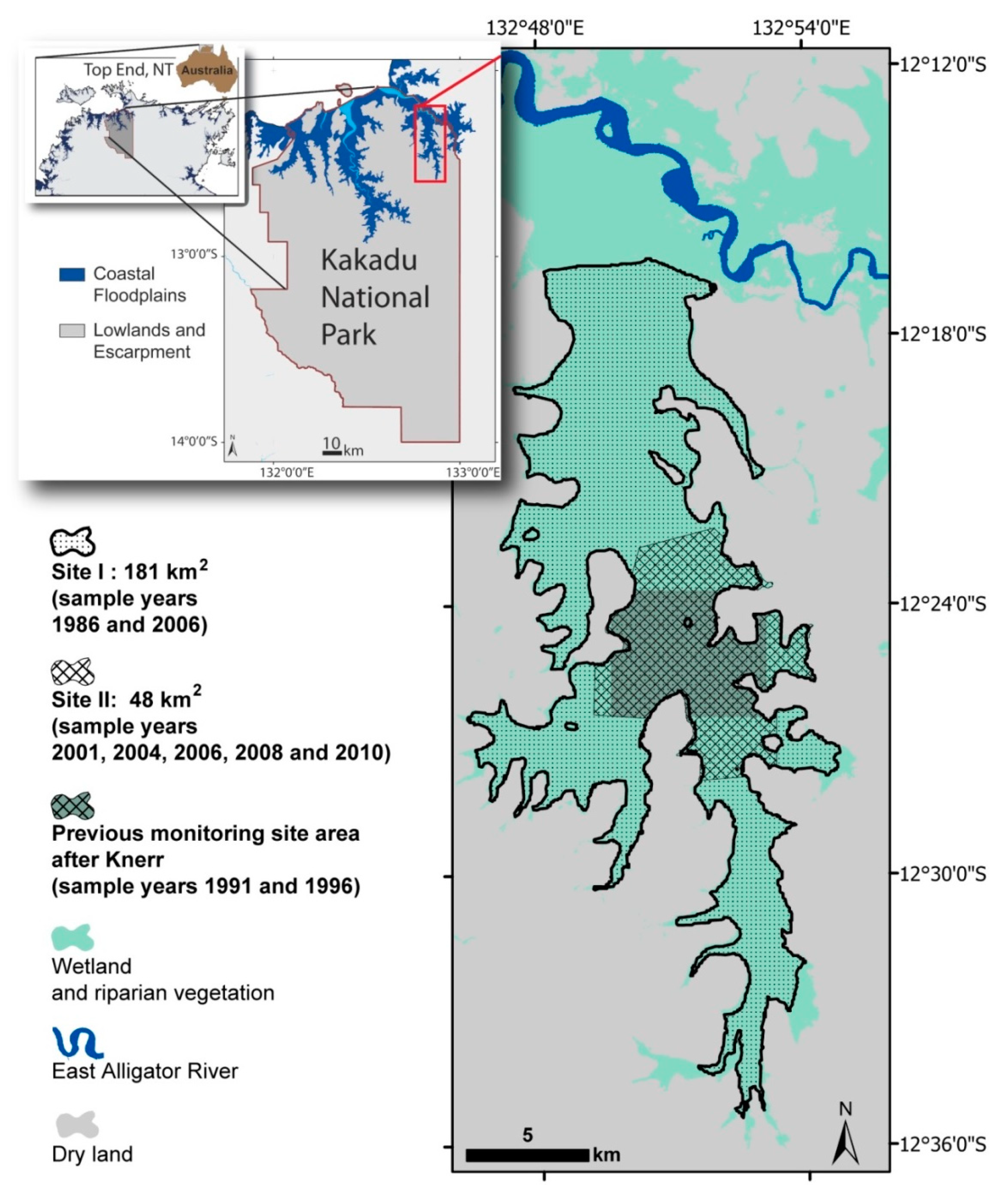
2.1. Site and Data Descriptions
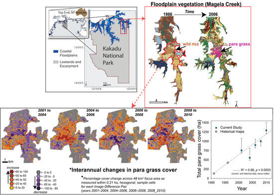
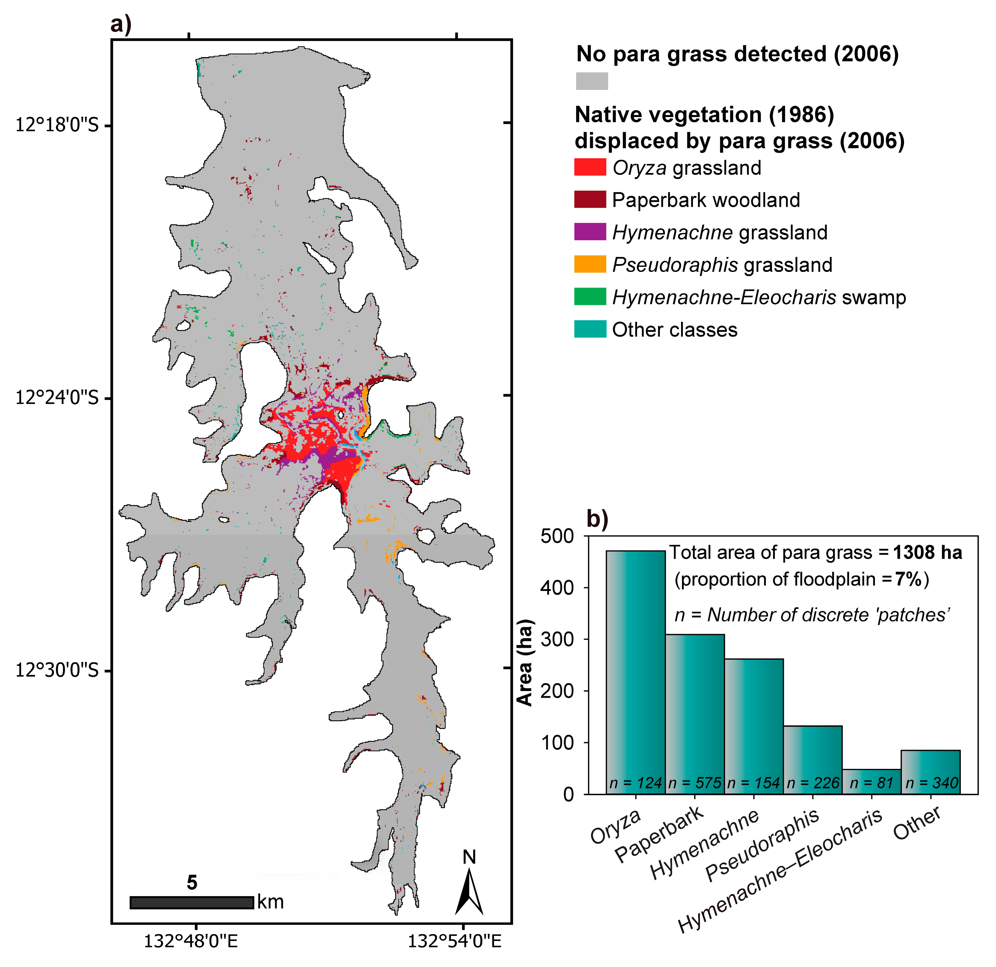
2.2. Native Vegetation Displaced by Para Grass from 1986 to 2006 (Site I)
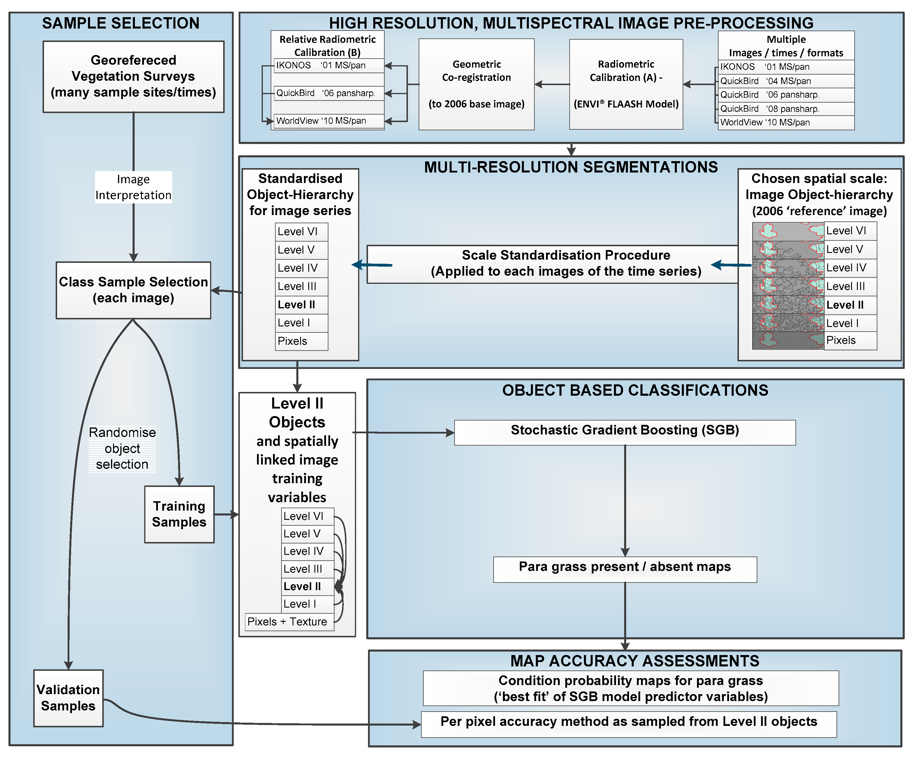
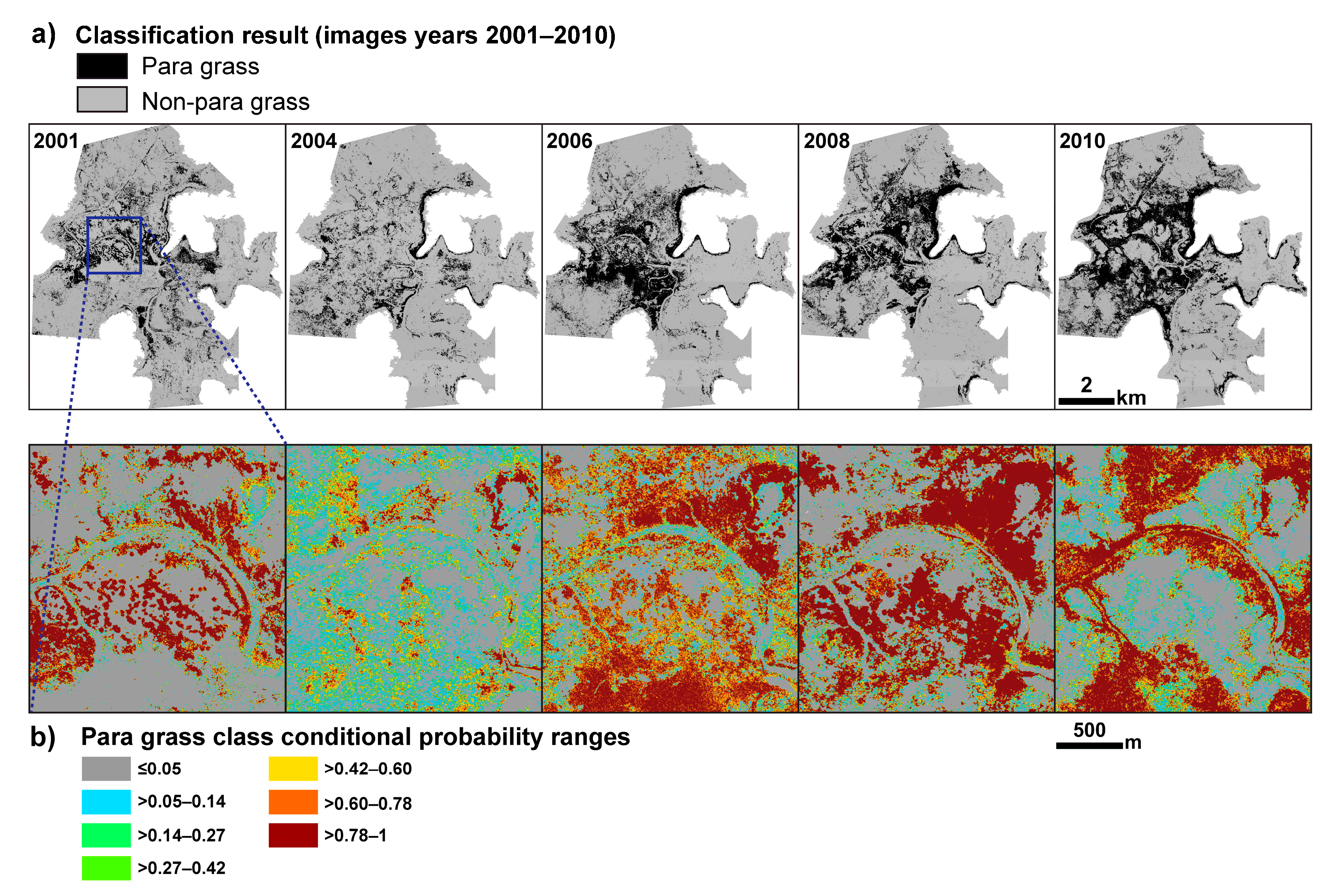
2.3. Production and Accuracy Assessment of Para Grass Map Series from 2001 to 2010 (Site II)
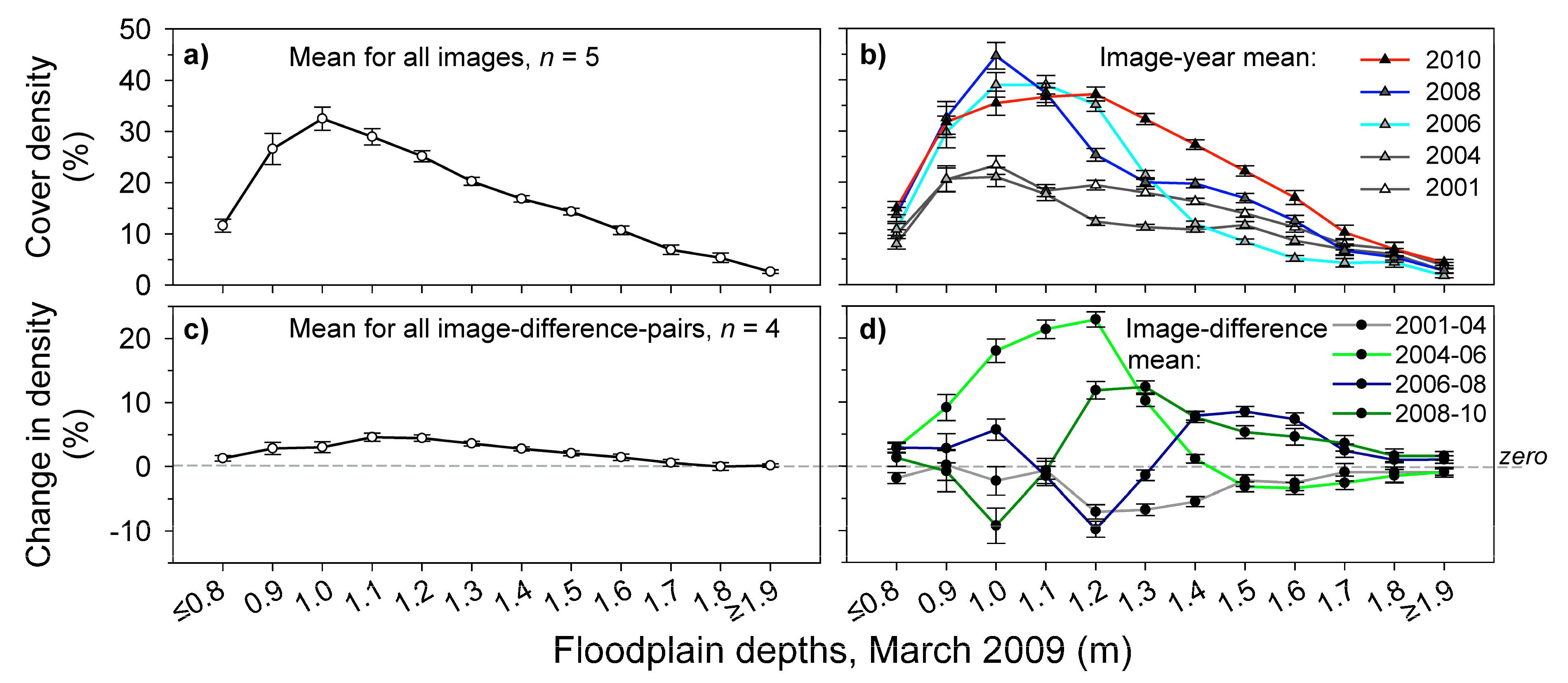
2.3.1. Estimating Trends and Variability in Para Grass Cover (Site II)
3. Results and Discussion
3.1. Native Vegetation Displaced by Para Grass from 1986 to 2006 (Site I)
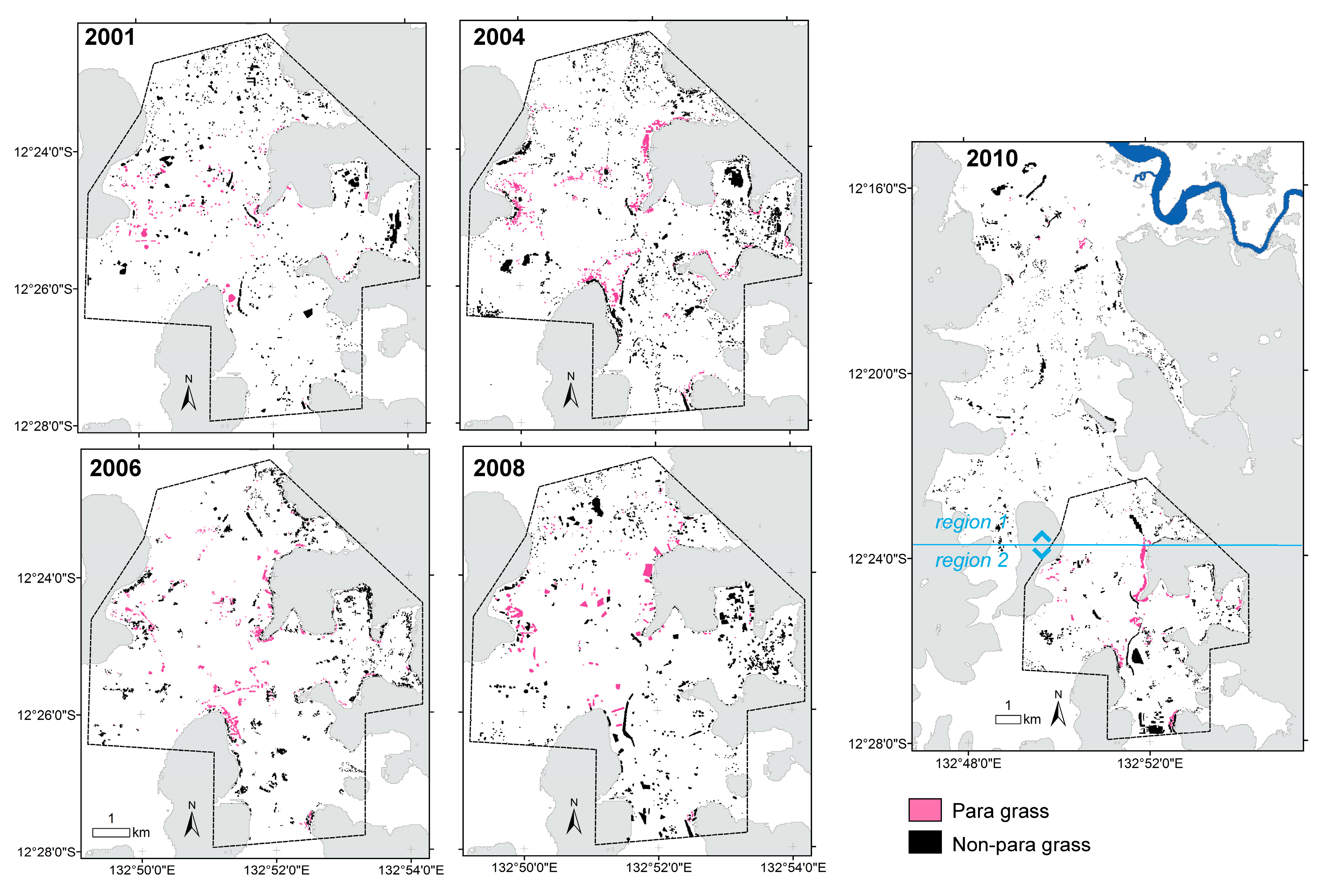
3.2. Production and Accuracy Assessment of Para Grass Map Series from 2001 to 2010 (Site II)
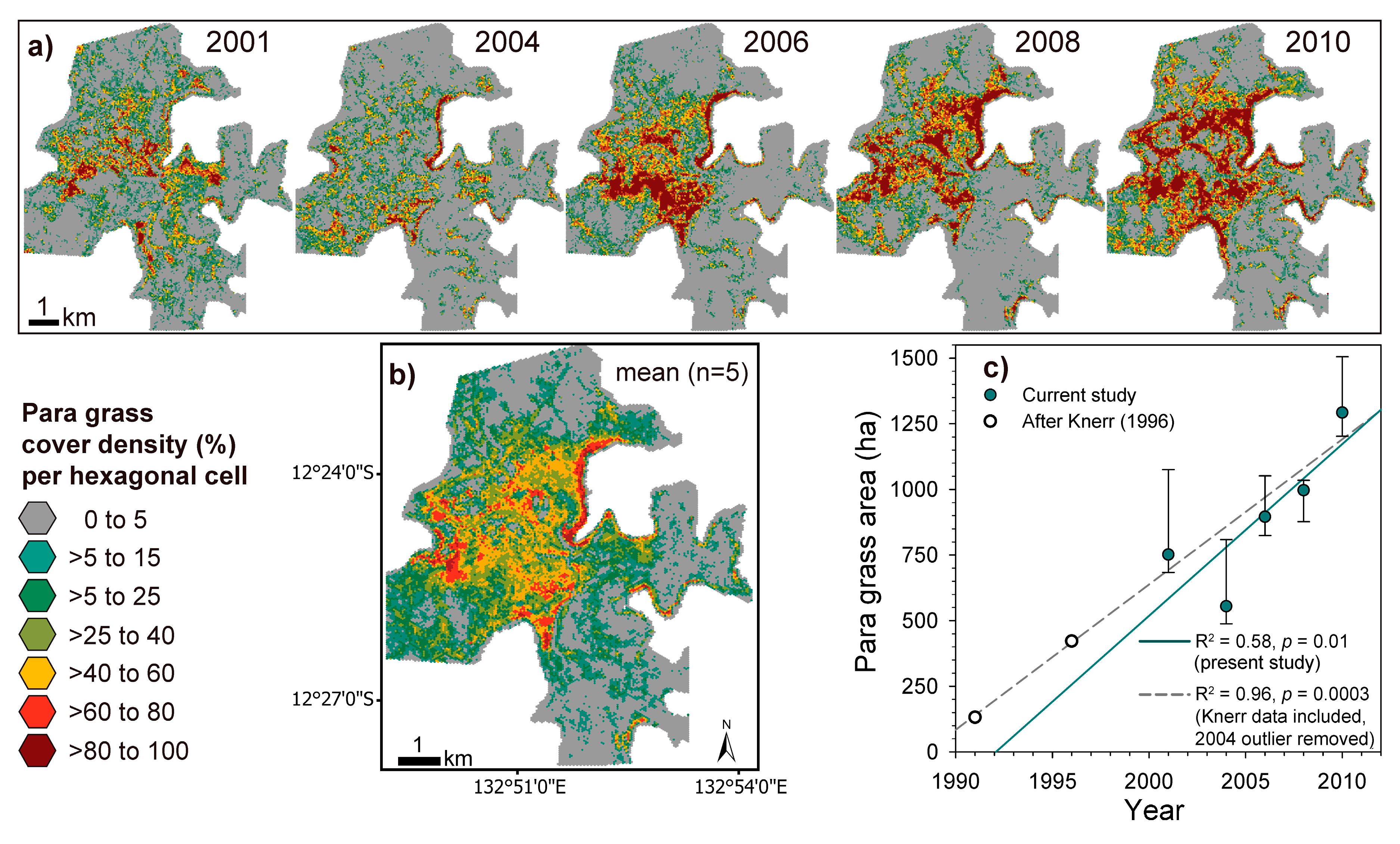
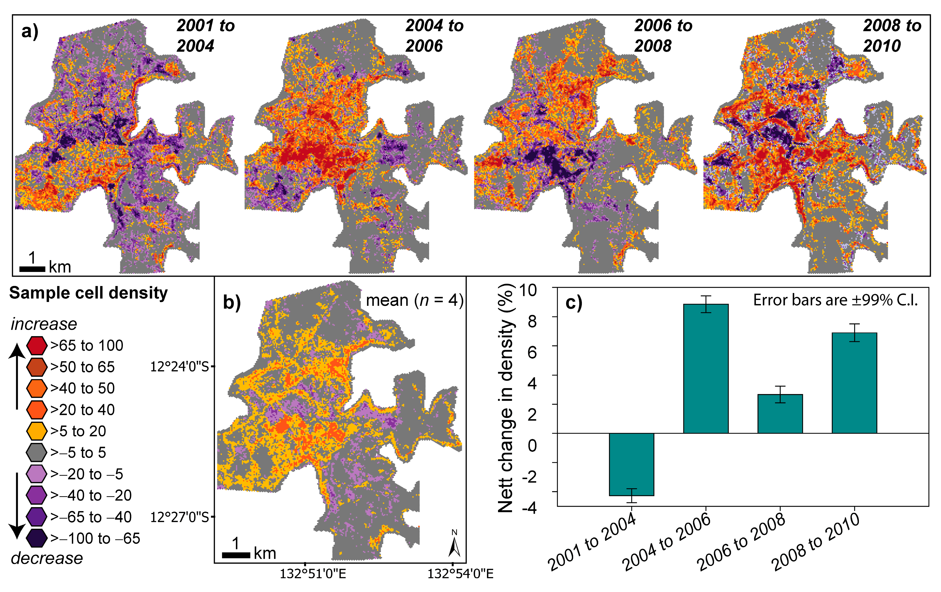
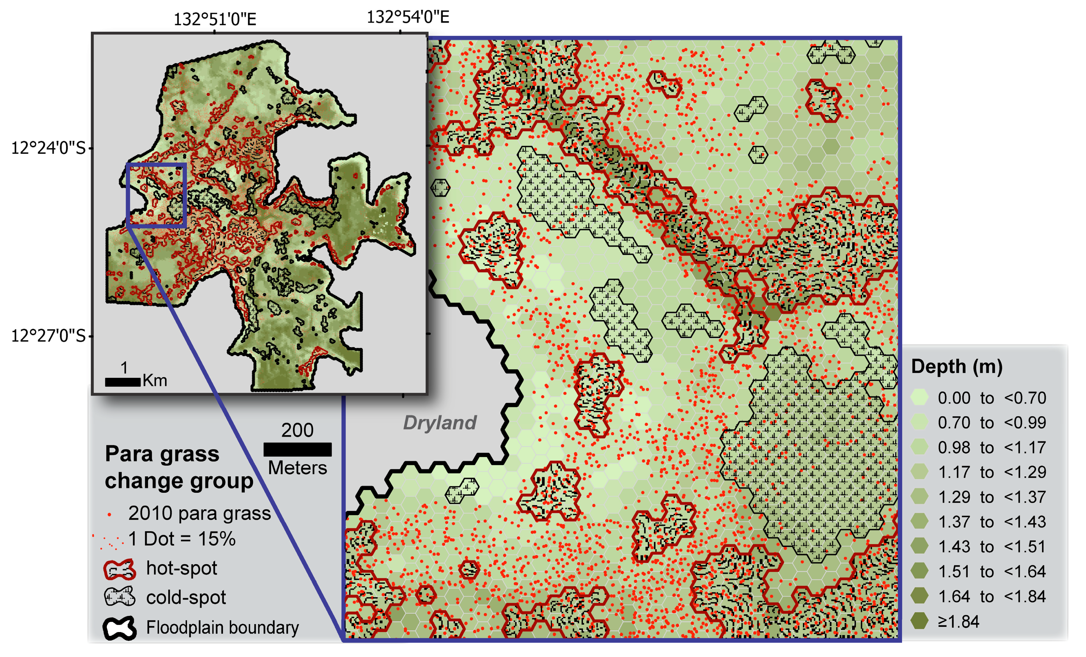
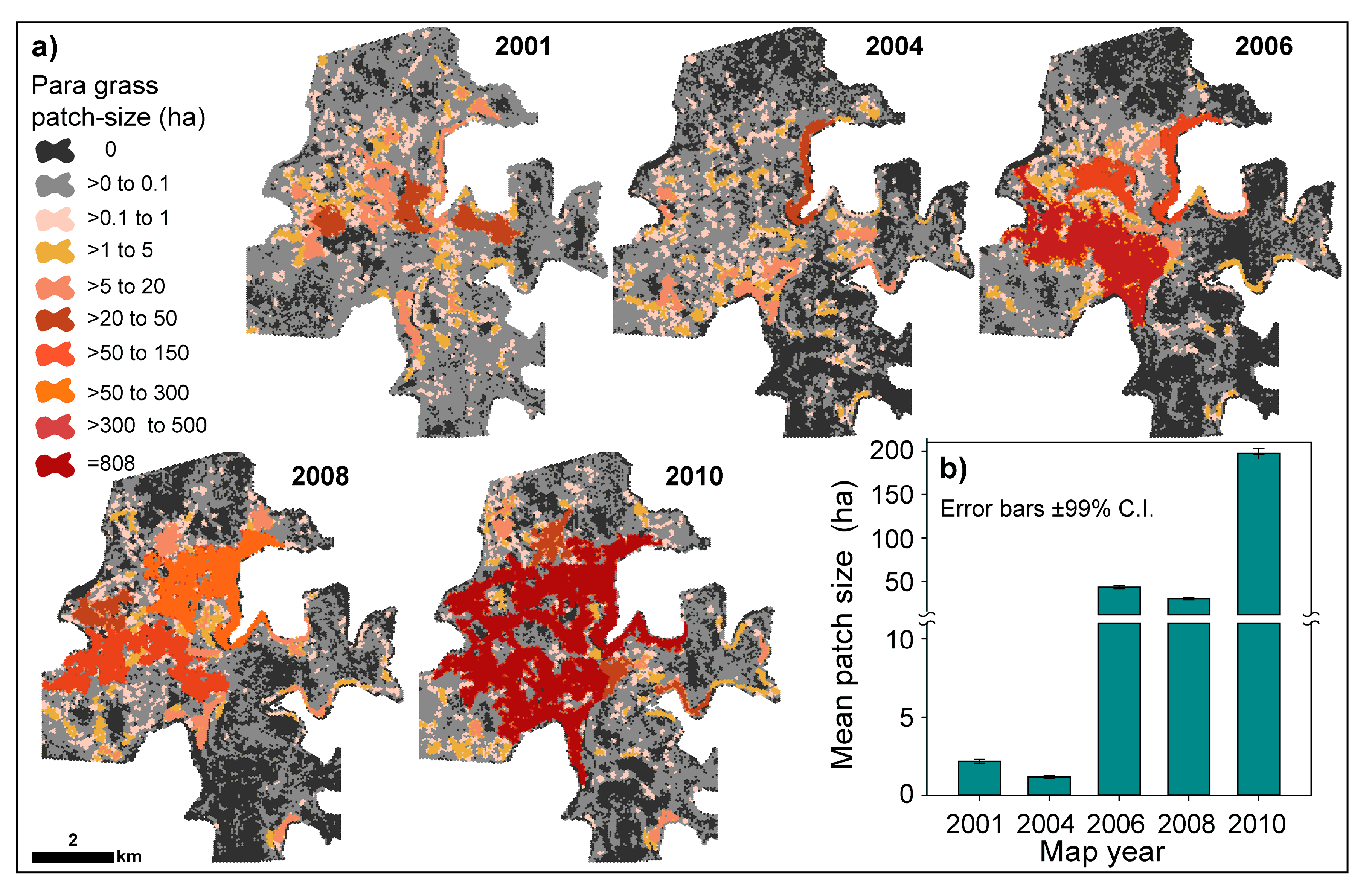
3.3. Measuring Distribution Trends and Inter-Annual Dynamics of Para Grass (Site II).
4. Conclusions
Author Contributions
Funding
Acknowledgments
Conflicts of Interest
References
- Assessment, M.E. Ecosystems and Human Well-Being: Wetlands and Water; World Resources Institute: Washington, DC, USA, 2005. [Google Scholar]
- Hu, S.; Niu, Z.; Chen, Y.; Li, L.; Zhang, H. Global wetlands: Potential distribution, wetland loss, and status. Sci. Total Environ. 2017, 586, 319–327. [Google Scholar] [CrossRef]
- Zedler, J.B.; Kercher, S. Causes and consequences of invasive plants in wetlands: Opportunities, opportunists, and outcomes. Crit. Rev. Plant Sci. 2004, 23, 431–452. [Google Scholar] [CrossRef]
- Kurugundla, C.; Mathangwane, B.; Sakuringwa, S.; Katorah, G. Alien Invasive Aquatic Plant Species in Botswana: Historical Perspective and Management. Open Plant Sci. J. 2016, 9. [Google Scholar] [CrossRef]
- Finlayson, C.; Gitay, H.; Bellio, M.; van Dam, R.; Taylor, I. Climate variability and change and other pressures on wetlands and waterbirds: Impacts and adaptation. In Waterbirds around the World: A Global Overview of the Conservation, Management and Research of the World’s Waterbird Flyways; The Stationery Office: London, UK, 2006; pp. 88–97. [Google Scholar]
- Low, T. Tropical pasture plants as weeds. Trop. Grassl. 1997, 31, 337–343. [Google Scholar]
- Bunn, S.E.; Davies, P.M.; Kellaway, D.M.; Prosser, I.P. Influence of invasive macrophytes on channel morphology and hydrology in an open tropical lowland stream, and potential control by riparian shading. Freshw. Biol. 1998, 39, 171–178. [Google Scholar] [CrossRef]
- Bellairs, S.M.; Wurm, P.A.S.; Kernich, B. Temperature affects the dormancy and germination of sympatric annual Oryza meridionalis and perennial O. rufipogon native Australian rices (Poaceae) and influences their emergence in introduced para grass Urochloa mutica swards. Aust. J. Bot. 2015, 63, 687–695. [Google Scholar] [CrossRef]
- Wurm, P. Suppression of germination and establishment of native annual rice by introduced para grass on an Australian monsoonal floodplain. Plant Prot. Q. 2007, 22, 106. [Google Scholar]
- Barrow, P. Fire management and research in Kakadu. In Supervising Scientist Report 148: A Compendium of Information for Managing and Monitoring Wetlands in Tropical Australia; Finlayson, C.M., Spiers, A.G., Eds.; Supervising Scientist: Canberra, Australia, 1999; pp. 198–206. [Google Scholar]
- Douglas, M.M.; O’Connor, R.A. Weed invasion changes fuel characteristics: Para grass (Urochloa mutica (Forssk.) T.Q. Nguyen) on a tropical floodplain. Ecol. Manag. Restor. 2004, 5, 143–145. [Google Scholar] [CrossRef]
- Finlayson, C.M. Plant ecology of Australia’s tropical floodplain wetlands: A review. Ann. Bot. 2005, 96, 541–555. [Google Scholar] [CrossRef]
- Finlayson, C.M.; Storrs, M.J.; Lindner, G. Degradation and rehabilitation of wetlands in the Alligator Rivers Region of northern Australia. Wetl. Ecol. Manag. 1997, 5, 19–36. [Google Scholar] [CrossRef]
- Setterfield, S.A.; Rossiter-Rachor, N.A.; Douglas, M.M.; Wainger, L.; Petty, A.M.; Barrow, P.; Shepherd, I.J.; Ferdinands, K.B. Adding fuel to the fire: The impacts of non-native grass invasion on fire management at a regional scale. PLoS ONE 2013, 8, e59144. [Google Scholar] [CrossRef] [PubMed]
- Finlayson, C.M.; Lowry, J.B.; Bellio, M.G.; Nou, S.; Pidgeon, R.; Walden, D.; Humphrey, C.; Fox, G. Biodiversity of wetlands of the Kakadu Region, northern Australia. Aquat. Sci. 2006, 68, 374–399. [Google Scholar] [CrossRef]
- Ferdinands, K.B.; Beggs, K.; Whitehead, P.J. Biodiversity and invasive grass species: Multiple-use or monoculture? Wildl. Res. 2005, 32, 447–457. [Google Scholar] [CrossRef]
- AVH. Australian Virtual Herbarium Occurrence Records: Urochloa Mutica. Available online: https://avh.chah.org.au/ (accessed on 28 August 2019).
- Ramsar. Convention on Wetlands of International Importance especially as Waterfowl Habitat. Ramsar (Iran). UN Treaty Series No. 14583. As amended in 1982 and 1987. Available online: http://www.ramsar.org/ (accessed on 28 August 2019).
- Knerr, N. Grassland Community Dynamics of a Freshwater Tropical Floodplain: Invasion of Brachiaria Mutica (Para Grass) on The Magela Floodplain, Kakadu National Park. Bachelor’s Thesis, University of New England, Armidale, NSW, Australia, 1996. [Google Scholar]
- Boyden, J.M.; Joyce, K.E.; Boggs, G.; Wurm, P. Object-based mapping of native vegetation and para grass (Urochloa mutica) on a monsoonal wetland of Kakadu NP using a Landsat 5 TM Dry-season time series. J. Spat. Sci. 2013, 58, 53–77. [Google Scholar] [CrossRef]
- Walden, D.; Boyden, J.; Bayliss, P.; Ferdinands, K. A preliminary ecological risk assessment of the major weeds on the Magela Creek floodplain, Kakadu National Park; Supervising Scientist Report 194; Supervising Scientist (Aust. Govt.): Darwin, NT, Australia, 2012; ISBN 978-1-921069-19-2.
- Whitehead, P.J.; Dawson, T. Let them eat grass. Nat. Aust. (Autumn) 2000, 45–55. [Google Scholar]
- Whitehead, P.J.; Wilson, B.A.; Bowman, D.M.J.S. Conservation status of coastal wetlands of the Northern Territory of Australia: The Mary River floodplain. Biol. Conserv. 1990, 52, 85–111. [Google Scholar] [CrossRef]
- Stein, J.C.; Yu, Y.; Copetti, D.; Zwickl, D.J.; Zhang, L.; Zhang, C.; Chougule, K.; Gao, D.; Iwata, A.; Goicoechea, J.L.; et al. Genomes of 13 domesticated and wild rice relatives highlight genetic conservation, turnover and innovation across the genus Oryza. Nat. Genet. 2018, 50, 285–296. [Google Scholar] [CrossRef]
- Hoang, T.M.L.; Tran, T.N.; Nguyen, T.K.T.; Williams, B.; Wurm, P.; Bellairs, S.; Mundree, S. Improvement of Salinity Stress Tolerance in Rice: Challenges and Opportunities. Agronomy 2016, 6, 54. [Google Scholar] [CrossRef]
- Frith, H.; Davies, S. Ecology of the Magpie Goose, Anseranas semipalmata Latham (Anatidae). CSIRO Wildl. Res. 1961, 6, 91–141. [Google Scholar] [CrossRef]
- Whitehead, P.J.; Saalfeld, K. Nesting phenology of magpie geese (Anseranas semipalmata) in monsoonal northern Australia: Responses to antecedent rainfall. J. Zool. 2000, 251, 495–508. [Google Scholar] [CrossRef]
- Redhead, T.D. On the demography of Rattus sordidus colletti in monsoonal Australia. Aust. J. Ecol. 1979, 4, 115–136. [Google Scholar] [CrossRef]
- Wurm, P. A surplus of seeds: High rates of post-dispersal seed predation in a flooded grassland in monsoonal Australia. Aust. J. Ecol. 1998, 23, 385–392. [Google Scholar] [CrossRef]
- McGregor, S.; Lawson, V.; Christophersen, P.; Kennett, R.; Boyden, J.M.; Bayliss, P.; Liedloff, A.; McKaige, B.; Andersen, A.N. Indigenous wetland burning: Conserving natural and cultural resources in Australia’s World Heritage-listed Kakadu National Park. Hum. Ecol. 2011, 32, 721–729. [Google Scholar] [CrossRef]
- Ligtermoet, E. Maintaining customary harvesting of freshwater resources: Sustainable Indigenous livelihoods in the floodplains of northern Australia. Rev. Fish Biol. Fish. 2016, 26, 649–678. [Google Scholar] [CrossRef]
- Vilà, M.; Ibáñez, I. Plant invasions in the landscape. Landsc. Ecol. 2011, 26, 461–472. [Google Scholar] [CrossRef]
- Catford, J.A.; Vesk, P.A.; White, M.D.; Wintle, B.A. Hotspots of plant invasion predicted by propagule pressure and ecosystem characteristics. Divers. Distrib. 2011, 17, 1099–1110. [Google Scholar] [CrossRef]
- Allen, C.; Johnson, A.; Parris, L. A Framework for Spatial Risk Assessments: Potential Impacts of Nonindigenous Invasive Species on Native Species. Ecol. Soc. 2006, 11, 39. [Google Scholar] [CrossRef]
- Hobbs, R.; Humphries, S. An integrated approach to the ecology and management of plant invasions. Conserv. Biol. 1995, 9, 761–770. [Google Scholar] [CrossRef]
- With, K.A. The landscape ecology of invasive spread. Conserv. Biol. 2002, 16, 1192–1203. [Google Scholar] [CrossRef]
- Rodgers, L.; Pernas, T.; Redwine, J.; Shamblin, B.; Bruscia, S. Multiscale Invasive Plant Monitoring: Experiences from the Greater Everglades Restoration Area. Weed Technol. 2018, 32, 11–19. [Google Scholar] [CrossRef]
- Levick, S.; Rogers, K. Context-dependent vegetation dynamics in an African savanna. Landsc. Ecol. 2011, 26, 515–528. [Google Scholar] [CrossRef]
- Randall, J.M.; Cole, D.; McCool, S.; Borrie, W. Improving management of nonnative invasive plants in wilderness and other natural areas. In Proceedings of the Wilderness Science in a Time of Change Conference-Volume 5: Wilderness Ecosystems, Threats, and Management, Missoula, MT, USA, 23–27 May 1999; U.S. Department of Agriculture, Forest Service, Rocky Mountain Research Station: Missoula, MT, USA, 2000; pp. 64–73. [Google Scholar]
- Harvey, K.R.; Hill, G.J.E. Vegetation mapping of a tropical freshwater swamp in the Northern Territory, Australia: A comparison of aerial photography, Landsat TM and SPOT satellite imagery. Int. J. Remote Sens. 2001, 22, 2911–2925. [Google Scholar] [CrossRef]
- D’Antonio, C.M.; Jackson, N.E.; Horvitz, C.C.; Hedberg, R. Invasive plants in wildland ecosystems: Merging the study of invasion processes with management needs. Front. Ecol. Environ. 2004, 2, 513–521. [Google Scholar] [CrossRef]
- Finlayson, C.M.; Rea, N. Reasons for the loss and degradation of Australian wetlands. Wetl. Ecol. Manag. 1999, 7, 1–11. [Google Scholar] [CrossRef]
- MacKay, H.; Finlayson, C.M.; Fernandez-Prieto, D.; Davidson, N.; Pritchard, D.; Rebelo, L.-M. The role of Earth Observation (EO) technologies in supporting implementation of the Ramsar Convention on Wetlands. J. Environ. Manag. 2009, 90, 2234–2242. [Google Scholar] [CrossRef] [PubMed]
- Sanderson, N.; Koontz, D.; Morley, A. The Ecology of the Vegetation of the Magela Creek Floodplain: Upper Section from Oenpelli Road Crossing to Nankeen Billabong. In Proceedings of the Scientific Workshop, Environmental Protection in the Alligator Rivers Region, Jabiru, Australia, 17–20 May 1983; pp. 17–20. [Google Scholar]
- Casanova, M.T.; Brock, M.A. How do depth, duration and frequency of flooding influence the establishment of wetland plant communities? Plant Ecol. 1983, 147, 237–250. [Google Scholar] [CrossRef]
- Finlayson, C.M. Vegetation changes and biomass on an Australian monsoonal floodplain. In Wetlands and Ecotones: Studies on Land-Water Interactions; Gopal, B., Hillbreicht-Ilkowska, A., Wetzel, R., Eds.; National Institute of Ecology and International Scientific Publications: New Delhi, Germany, 1993; pp. 157–172. [Google Scholar]
- Middleton, B. Succession and herbivory in monsoonal wetlands. Wetl. Ecol. Manag. 1999, 6, 189–202. [Google Scholar] [CrossRef]
- Ngari, A.N.; Kinyamario, J.I.; Ntiba, M.J.; Mavuti, K.M. Factors affecting abundance and distribution of submerged and floating macrophytes in Lake Naivasha, Kenya. Afr. J. Ecol. 2009, 47, 32–39. [Google Scholar] [CrossRef]
- Peters, J. Ecohydrology of Wetlands: Monitoring and Modelling Interactions Between Groundwater, Soil and Vegetation. Ph.D. Thesis, Faculty of Bioscience Engineering, Ghent University, Ghent, Belgium, 2008. [Google Scholar]
- Whitehead, P.J.; Russell-Smith, J.; Woinarski, J.C.Z. Fire, landscape heterogeneity and wildlife management in Australia’s tropical savannas: Introduction and overview. Wildl. Res. 2008, 32, 369–375. [Google Scholar] [CrossRef]
- Boyden, J.; Wurm, P.; Joyce, K.E.; Boggs, G. A spatial vulnerability assessment of monsoonal wetland habitats to para grass invasion in Kakadu National Park, northern Australia. Int. J. Appl. Earth Obs. Geoinf. 2018, 71, 43–55. [Google Scholar] [CrossRef]
- Ward, D.P.; Petty, A.M.; Setterfield, S.A.; Douglas, M.M.; Ferdinands, K.B.; Hamilton, S.K.; Phinn, S.R. Floodplain inundation and vegetation dynamics in the Alligator Rivers region (Kakadu) of northern Australia assessed using optical and radar remote sensing. Remote Sens. Environ. 2014, 147, 43–55. [Google Scholar] [CrossRef]
- Williams, P.R.; Collins, E.M.; Grice, A.C.; Mike Nicholas, D.; Perry, J.J. The role of fire in germinating wild rice (Oryza meridionalis), an annual grass of northern Australian wetlands threatened by exotic grass invasion. Ecol. Manag. Restor. 2011, 12, 74–76. [Google Scholar] [CrossRef]
- Grice, A.; Nicholas, M. Using fire to restore Australian wetlands from invasive grasses, Rural Industries Research and Development Corporation. Aust. Gov. 2011, 11. [Google Scholar]
- Hobbs, R.; Huenneke, L. Disturbance, diversity, and invasion: Implications for conservation (review). Conserv. Biol. 1992, 6, 324–337. [Google Scholar] [CrossRef]
- Wallace, J.; Caccetta, P.A.; Kiiver, H.T. Recent developments in analysis of spatial and temporal data for landscape qualities and monitoring. Austral Ecol. 2004, 29, 100–107. [Google Scholar] [CrossRef]
- Dronova, I.; Knox, S.H.; Taddeo, S.; Hemes, K.S.; Valach, A.C.; Oikawa, P.; Baldocchi, D.D. The potential of remotely sensed phenology as indicator of structure and function in wetland ecosystems (356823). In Proceedings of the 2018 AGU Fall Meeting, Washington, DC, USA, 10–14 December 2018. [Google Scholar]
- Dronova, I.; Spotswood, E.N.; Suding, K.N. Opportunities and Constraints in Characterizing Landscape Distribution of an Invasive Grass from Very High Resolution Multi-Spectral Imagery. Front. Plant Sci. 2017, 8, 890. [Google Scholar] [CrossRef] [PubMed]
- Dronova, I.; Gong, P.; Wang, L.; Zhong, L. Mapping dynamic cover types in a large seasonally flooded wetland using extended principal component analysis and object-based classification. Remote Sens. Environ. 2015, 158, 193–206. [Google Scholar] [CrossRef]
- Boyden, J.M.; Walden, D.; Bartolo, R.; Bayliss, P. Utility of VHR remote sensing data for landscape scale assessment of the environmental weed, para grass [Urochloa mutica, (FORSSK), Nguyen], on a tropical floodplain. In Proceedings of the 28th Asian Conference on Remote Sensing, Kuala, Lumpur, 12–16 November 2008. [Google Scholar]
- Becker, B.L.; Lusch, D.P.; Qi, J. A classification-based assessment of the optimal spectral and spatial resolutions for Great Lakes coastal wetland imagery. Remote Sens. Environ. 2007, 108, 111–120. [Google Scholar] [CrossRef]
- De Roeck, E.; Verhoest, N.; Miya, M.; Lievens, H.; Batelaan, O.; Thomas, A.; Brendonck, L. Remote sensing and wetland ecology: A South African case study. Sensors 2008, 8, 3542–3556. [Google Scholar] [CrossRef]
- Dronova, I.; Gong, P.; Wang, L. Object-based analysis and change detection of major wetland cover types and their classification uncertainty during the low water period at Poyang Lake, China. Remote Sens. Environ. 2011, 115, 3220–3236. [Google Scholar] [CrossRef]
- Johnston, R.; Barson, M. Remote sensing of Australian wetlands: An evaluation of Landsat TM data for inventory and classification. Aust. J. Mar. Freshw. Res. 1993, 44, 235–252. [Google Scholar] [CrossRef]
- Klemas, V. Remote sensing of wetlands: Case studies comparing practical techniques. J. Coast. Res. 2011, 27, 418–427. [Google Scholar]
- Laba, M.; Downs, R.; Smith, S.; Welsh, S.; Neider, C.; White, S.; Richmond, M.; Philpot, W.; Baveye, P. Mapping invasive wetland plants in the Hudson River National Estuarine Research Reserve using QuickBird satellite imagery. Remote Sens. Environ. 2008, 112, 286–300. [Google Scholar] [CrossRef]
- Lunetta, R.; Balogh, M. Application of multi-temporal Landsat 5 TM imagery for wetland Identification. Photogramm. Eng. Remote Sens. 1999, 65, 1303–1310. [Google Scholar]
- Olmanson, L.G.; Bauer, M.E.; Brezonik, P.L. Aquatic vegetation surveys using high-resolution IKONOS imagery. In Proceedings of the 15th William T. Pecora Memorial Remote Sensing Symposium; Unpaginated CD ROM: Denver, CO, USA, 2002; p. 5. [Google Scholar]
- Ozesmi, S.L.; Bauer, M.E. Satellite remote sensing of wetlands. Wetl. Ecol. Manag. 2002, 10, 381–402. [Google Scholar] [CrossRef]
- Ward, D.P.; Hamilton, S.K.; Jardine, T.D.; Pettit, N.E.; Tews, E.K.; Olley, J.M.; Bunn, S.E. Assessing the seasonal dynamics of inundation, turbidity, and aquatic vegetation in the Australian wet–dry tropics using optical remote sensing. Ecohydrology 2012, 6, 312–323. [Google Scholar] [CrossRef]
- Gillanders, S.N.; Coops, N.C.; Wulder, M.A.; Gergel, S.E.; Nelson, T. Multitemporal remote sensing of landscape dynamics and pattern change: Describing natural and anthropogenic trends. Prog. Phys. Geography 2008, 32, 503–528. [Google Scholar] [CrossRef]
- Shaw, D. Translation of remote sensing data into weed management decisions. Weed Sci. 2005, 53, 264–273. [Google Scholar] [CrossRef]
- Kennedy, R.E.; Townsend, P.A.; Gross, J.E.; Cohen, W.B.; Bolstad, P.; Wang, Y.Q.; Adams, P. Remote sensing change detection tools for natural resource managers: Understanding concepts and tradeoffs in the design of landscape monitoring projects. Remote Sens. Environ. 2009, 113, 1382–1396. [Google Scholar] [CrossRef]
- Abeysinghe, T.; Simic Milas, A.; Arend, K.; Hohman, B.; Reil, P.; Gregory, A.; Vázquez-Ortega, A. Mapping Invasive Phragmites australis in the Old Woman Creek Estuary Using UAV Remote Sensing and Machine Learning Classifiers. Remote Sens. 2019, 11, 1380. [Google Scholar] [CrossRef]
- Whiteside, T.G.; Bartolo, R.E. Mapping Aquatic Vegetation in a Tropical Wetland Using High Spatial Resolution Multispectral Satellite Imagery. Remote Sens. 2015, 7, 11664–11694. [Google Scholar] [CrossRef] [Green Version]
- Gray, P.; Ridge, J.; Poulin, S.; Seymour, A.; Schwantes, A.; Swenson, J.; Johnston, D. Integrating drone imagery into high resolution satellite remote sensing assessments of estuarine environments. Remote Sens. 2018, 10, 1257. [Google Scholar] [CrossRef]
- Shao, G.; Wu, J. On the accuracy of landscape pattern analysis using remote sensing data. Landsc. Ecol. 2008, 23, 505–511. [Google Scholar] [CrossRef]
- Lunetta, R. Chapter 1: Applications, project formulation, and analytical approach. In Remote Sensing Change Detection: Environmental Monitoring Methods and Applications; Lunetta, R., Elvidge, C., Eds.; Ann Arbor Press: Michigan, MI, USA, 1998; pp. 1–20. [Google Scholar]
- Coppin, P.; Jonkheere, I.; Nackaerts, K.; Muys, B. Digital change detection methods in ecosystem monitoring: A review. Int. J. Remote Sens. 2004, 25, 1565–1596. [Google Scholar] [CrossRef]
- Salau, R. Para Grass in Kakadu National Park: Unpublished Paper Presented to Natural Resource Management Canberra; Australian Nature Conservation Agency: Canberra, Australia, 1995. [Google Scholar]
- Wesley-Smith, R. Para grass in the Northern Territory: Parentage and propagation. Trop. Grassl. 1973, 7, 249–250. [Google Scholar]
- Petty, A.M.; Werner, P.A.; Lehmann, C.E.R.; Riley, J.E.; Banfai, D.S.; Elliott, L.P. Savanna responses to feral buffalo in Kakadu National Park, Australia. Ecol. Monogr. 2007, 77, 441–463. [Google Scholar] [CrossRef]
- Finlayson, C.M.; Bailey, B.J.; Cowie, I.D. Macrophyte vegetation of the Magela Creek flood plain, Alligator Rivers Region, Northern Territory. In Research Report 5; Supervising Scientist for the Alligator Rivers Region: Canberra, Australia, 1989. [Google Scholar]
- Pfitzner, K. IKONOS and ASTER Imagery: Ranger Mine and the Magela Floodplain Area; Supervising Scientist: Darwin, Australia, 2003. [Google Scholar]
- Excelis. ENVI User Manual; ITT Visual Information Solutions: Boulder CO, USA, 2010. [Google Scholar]
- Trimble. Reference Book: eCognition® Developer 8.64.1; Trimble Germany GmbH: Trappentreustr. 1, D-80339 München, Germany, 2011. [Google Scholar]
- ESRI. ArcMap Version 9.3.1; Environmental Systems Research Institute, Inc. (ESRI): Redlands, CA, USA, 2006. [Google Scholar]
- Boyden, J. Remote Sensing Applications: Understanding the Landscape Ecology of Invasive Para Grass (urochloa mutica) on Monsoonal Wetlands, Kakadu National Park, Australia. Ph.D. Thesis, Charles Darwin University, Darwin, Australia, 2016. [Google Scholar]
- Baker, C.; Lawrence, R.; Montagne, C.; Patten, D. Change detection of wetland ecosystems using Landsat imagery and change vector analysis. Wetlands 2007, 27, 610–619. [Google Scholar] [CrossRef]
- Lawrence, R.; Bunn, A.; Powell, S.; Zambon, M. Classification of remotely sensed imagery using stochastic gradient boosting as a refinement of classification tree analysis. Remote Sens. Environ. 2004, 90, 331–336. [Google Scholar] [CrossRef]
- McIver, D.K.; Friedl, M.A. Using prior probabilities in decision-tree classification of remotely sensed data. Remote Sens. Environ. 2002, 81, 253–261. [Google Scholar] [CrossRef]
- Zhu, X. Wetland mapping using remote sensing imagery and ModelMap. In Proceedings of the Surveying and Spatial Science Biennial Conference, Wellington, New Zealand, 21–25 November 2011. [Google Scholar]
- Friedman, J. Stochastic gradient boosting. Comput. Stat. Data Anal. 2002, 38, 367–378. [Google Scholar] [CrossRef]
- Friedman, J Greedy function approximation: A gradient boosting machine. Ann. Stat. 2001, 29, 1189–1232. [CrossRef]
- Friedman, J.; Hastie, T.; Tibshirani, R. Special invited paper. Additive logistic regression: A statistical view of boosting. Ann. Stat. 2000, 28, 337–374. [Google Scholar] [CrossRef]
- Kim, H.-C.; Pang, S.; Je, H.-M.; Kim, D.; Bang, S.Y. Constructing support vector machine ensemble. Pattern Recognit. 2003, 36, 2757–2767. [Google Scholar] [CrossRef]
- Elith, J.; Leathwick, J.R.; Hastie, T. A working guide to boosted regression trees. J. Anim. Ecol. 2008, 77, 802–813. [Google Scholar] [CrossRef] [PubMed]
- Andrew, M.E.; Ustin, S.L. The role of environmental context in mapping invasive plants with hyperspectral image data. Remote Sens. Environ. 2008, 112, 4301–4317. [Google Scholar] [CrossRef]
- Lu, D.; Weng, Q. A survey of image classification methods and techniques for improving classification performance. Int. J. Remote Sens. 2007, 28, 823–870. [Google Scholar] [CrossRef]
- StatSoft-Inc. Statistica 64 ver. 11 (data Analysis Software System). Available online: http://www.statsoft.com (accessed on 28 August 2019).
- Lewin-Koh, N. Hexagonal Binning: An overview. 14 May 2019. Available online: http://cran. r-project. org/web/packages/hexbin/vignettes/hexagon_binning. pdf (accessed on 28 August 2019).
- Carr, D.B.; Olsen, A.R.; White, D. Hexagon mosaic maps for display of univariate and bivariate geographical data. Cartogr. Geogr. Inf. Sci. 1992, 19, 228–236. [Google Scholar] [CrossRef]
- Anselin, L. Local indicators of spatial association—LISA. Geogr. Anal. 1995, 27, 93–115. [Google Scholar] [CrossRef]
- Ferdinands, K.B. Assessing the Threat Posed by an Invasive African Grass Urochloa Mutica (Forssk) Nguyen to Biodiversity Conservation in the Mary River Wetlands, Northern Territory. Ph.D. Thesis, Charles Darwin University, Darwin, Australia, 2007. [Google Scholar]
- Douglas, M.M.; O’Connor, R.A. Effects of the exotic macrophyte, para grass (Urochloa mutica), on benthic and epiphytic macroinvertebrates of a tropical floodplain. Freshw. Biol. 2003, 48, 962–971. [Google Scholar] [CrossRef]
- Douglas, M.M.; Bunn, S.E.; Pidgeon, R.J.; Davies, P.M.; Barrow, P.; O’Connor, R.A.; Winning, M. Weed Management and the Biodiversity and Ecological Processes of Tropical Wetlands; Final Report; National Wetlands, R.& D Program, Environment Australia & Land and Water Australia: Canberra, ACT, Australia, 2001. [Google Scholar]
- Setterfield, S.A.; Clifton, P.J.; Hutley, L.B.; Rossiter-Rachor, N.A.; Douglas, M.M. Exotic grass invasion alters microsite conditions limiting woody recruitment potential in an Australian savanna. Sci. Rep. 2018, 8, 6628. [Google Scholar] [CrossRef] [Green Version]
- Heinl, M.; Sliva, J.; Murray-Hudson, M.; Tacheba, B. Post-fire succession on savanna habitats in the Okavango Delta wetland, Botswana. J. Trop. Ecol. 2007, 23, 705–713. [Google Scholar] [CrossRef]
- Lechner, A.M.; Stein, A.; Jones, S.D.; Ferwerda, J.G. Remote sensing of small and linear features: Quantifying the effects of patch size and length, grid position and detectability on land cover mapping. Remote Sens. Environ. 2009, 113, 2194–2204. [Google Scholar] [CrossRef]
- Johnston, C.A.; Bridgham, S.D.; Schubauer-Berigan, J.P. Nutrient dynamics in relation to geomorphology of riverine wetlands research funded by the USDA national research initiative competitive grants program (92-37102-7406). Contribution No. 240 of the center for water and the environment. Soil Sci. Soc. Am. J. 2001, 65, 557–577. [Google Scholar] [CrossRef]
- Chaudhari, S.; Sellers, B.A.; Rockwood, S.V.; Ferrell, J.A.; MacDonald, G.E.; Kenworthy, K.E. Nonchemical methods for para grass (Urochloa mutica) control. Invasive Plant Sci. Manag. 2012, 5, 20–26. [Google Scholar] [CrossRef]
- BoM. Climate statistics for Australian Locations: Monthy climate Statistics for Oenpelli and East Alligator Ranger Stations, Northern Territory, Australia (Weaterh Station Numbers 14042, 14293). Available online: http://www.bom.gov.au/climate/averages/tables/cw_014042_All.shtml (accessed on 25 June 2013).
- Lunetta, R.; Iiames, J.; Knight, J.; Congalton, R.; Mace, T. An assessment of reference data variability using a ‘virtual field reference database’. Photogramm. Eng. Remote Sens. 2001, 63, 707–715. [Google Scholar]
- Stone, K.R. Urochloa Mutica. In Fire Effects Information System; U.S. Department of Agriculture, Forest Service, Rocky Mountain Research Station, Fire Sciences Laboratory (Producer): Lakewood, CO, USA, 2010. [Google Scholar]
- Chesson, P. Mechanisms of maintenance of species diversity. Annu. Rev. Ecol. Syst. 2000, 31, 343–366. [Google Scholar] [CrossRef]
- Daehler, C. Performance comparisons of co-occurring native and alien invasive plants: Implications for conservation and restoration. Annu. Rev. Ecol. Evol. Syst. 2003, 34, 183–211. [Google Scholar] [CrossRef]
- Chadhokar, P. Effective rate and frequency of nitrogen applcations on dry matter yield and nitrogen content of para grass (Brachiaria mutica). Trop. Grassl. 1978, 12, 127–132. [Google Scholar]
- Whitehead, P.J.; McGuffog, T. Fire and vegetation pattern in tropical floodplain grassland: A description from the Mary River and its implications for wetland management. In Proceedings of the Australian Bushfire Conference, Plaza Hotel, Darwin, NT, Australia, 8–10 July 1997; pp. 115–121. [Google Scholar]
- Saxena, A.K.; Rana, B.S.; Rao, O.P.; Singh, B.P. Seasonal variation in biomass and primary productivity of para grass (Brachiaria mutica) under a mixed tree stand and in an adjacent open area in northern India. Agrofor. Syst. 1996, 33, 75–85. [Google Scholar] [CrossRef]
- Finlayson, C.M. Production and major nutrient composition of three grass species on the Magela floodplain, Northern Territory, Australia. Aquat. Bot. 1991, 41, 263–280. [Google Scholar] [CrossRef]
- Grice, A.; Perry, J.; Nicholas, D.; Williams, P. Managing complexity: The example of invasive wetland forage grasses. In 16th Australian Weeds Conference Proceedings: Weed Management 2008 Hot Topics in the Tropics; van Klinken, R., Osten, V., Panetta, P., Scanlan, J., Eds.; Queensland Weeds Society: Queensland, Australia, 2008; pp. 27–29. [Google Scholar]
- US EPA. Guidelines for ecological risk assessment. In Risk Assessment Forum; Environmental Protection Agency: Washington, DC, USA, 1998. [Google Scholar]
- Boyden, J.M.; Walden, D.; Bayliss, P.; Saalfeld, K. A GIS Compendium for Landscape-Scale Risk Assessment of the Magela Creek Floodplain and Broader Alligator Rivers Region, NT; Supervising Scientist: Darwin NT, Australia, 2008. [Google Scholar]


| Site Analyses | Map Variable | Mapping Year(s) | Description | Estimated Scale/Accuracy |
|---|---|---|---|---|
| Broad scale, generalized, analyses (Site I) | Para grass cover | 2006 | Published vegetation map produced by object-based image analysis from 2006 Landsat multi-temporal (dry season) composite using the Nearest Neighbour classifier [20]. | Horizontal accuracy ± 30 m. Overall accuracy for para grass cover class = 96% |
| Native vegetation cover | 1986 | Published vegetation map produced by aerial photo interpretation from 1:25000 images, in conjunction with georeferenced field knowledge. [83]. | Quantitative accuracy of the original map is unmeasured. Map digitized and spatially co-registered to 2006 map (Section 2.2). | |
| Finer-scale, inter-annual, analyses (Site II) | Para grass cover | 2001, 2004,2006, 2008, 2010 | This map series was produce from high spatial resolution satellite imagery (Table 2) using a supervised, object-based, classification (Section 2.3). Map accuracies were estimated using separate image samples reserved for validation. | Imagery/maps spatially co-registered to an accurately georectified (2006 QuickBird imagery) with horizontal accuracy approximately ± 2.5 m. Overall classification accuracies were ≥96% (Table 3, results). |
| Para grass Cover | 1991, 1996 | Map produced by aerial photo interpretation of 1:25000 images, with georeferenced ground surveys of vegetation used to validate interpretations. Published methods [19]. | Quantitative accuracy of the original imagery/maps is unmeasured. | |
| Water Depth | 2006 | A depth model of site I, extracted for Site II analyses. Modeled by regression between a Landsat dry-season composite and georefereced floodplain depth records. Published methods [51]. | Horizontal accuracy ± 30 m. Depth prediction strength R2 = 0.67, p < 0.0001, n = 254. Mapped at a spatial resolution of 30 m. Predicted depths ranged from 0 to 1.85 m in increments of 0.1 m. | |
| Fire Scar maps | 2000, 2003, 2005, 2007, 2009 | Maps produced by object-based image analysis of Landsat (available dry-season imagery) using the Nearest Neighbour classifier. Published methods [51]. | Horizontal accuracy ± 30 m pixels. Overall classification accuracies for map series: 98%, 99.6%, 93%, 99% and 99% respectively. |
| Sensor | Spatial Resolution | Analysis Resolution | Spectral Characteristics | Acquisition Date(s) | Additional Notes |
|---|---|---|---|---|---|
| IKONOS | Pixel size: 0.8 m (pan) 4 m (MS) All bands were provided at 1 m | 0.6 m | Band 1: 445–516 nm (Blue) Band 2: 506–595 nm (Green) Band 3: 632–698 nm (Red) Band 4: 757–853 nm (Near-IR) Pan: 450–900 nm Dynamic range: 11 bit | 03-06-2001 | Data geo-rectified and resampled to 1 m [84] |
| QuickBird | Pixel size: 0.6 m (pan and pan-sharped bands), 2.4 m (MS) | 0.6 m | Band 1: 450–520 nm (Blue) Band 2: 520–600 nm (Green) Band 3: 630–690 nm (Red) Band 4: 760–900 nm (Near-IR) Pan: 445–900 nm Dynamic range: 11 bit | 25-06-2004 | panchromatic + 4-band multispectral product |
| 23-06-2006 24-07-2006 | 4-band, UNB-pan-sharpened mosaic geo-rectified to ground control and used as the base image for spatial co-registration | ||||
| 15-06-2008 | UNB-pansharpened | ||||
| WorldView-2 | Pixel size: 0.49 m (pan) 2.4 m (MS) | 0.6 m | Band 1 *: 400–450 nm (Coastal) Band 2: 450–510 nm (Blue) Band 3: 510–580 nm (Green) Band 4 *: 585–625 nm (Yellow) Band 5: 630–690 nm (Red) Band 6 *: 705–745 nm (Red-edge) Band 7: 770–895 nm (Near-IR-1) Band 8 *: 860–900 nm (Near-IR-2) Pan: 450–800 nm | 15-05-2010 | panchromatic + 8-band multispectral product. Two separate scenes (Region 1 and 2), |
| Model Training Class | Sampled Vegetation Cover Types |
|---|---|
| Para grass | Urochloa mutica: dense cover, near mono-culture—wet and dry phases |
| Non-para grass | Native perennial grasses and floating vegetation mats: Dense vegetative cover dominated by Hymenachne acutigluma or Leersi hexandra |
| Annual grasses and sparse native perennial grasses, and ephemeral sedges: Oryza meriondalis, Pseudoraphis spinecens and E. dulcis (native rice, mud-grass and water chestnut) | |
| Non-floodplain grasses and bare ground | |
| Sedges: Dense vegetative cover of perennial and ephemeral sedges (e.g., Eleocharis sphacelata and E. dulcis) | |
| Open water Lilies dominated by Nymphaea or Nymphoides spp. | |
| Nelumbo nucifera (red lily) | |
| Melaleuca (paperbark trees) | |
| Deeper open water with no emergent vegetation cover |
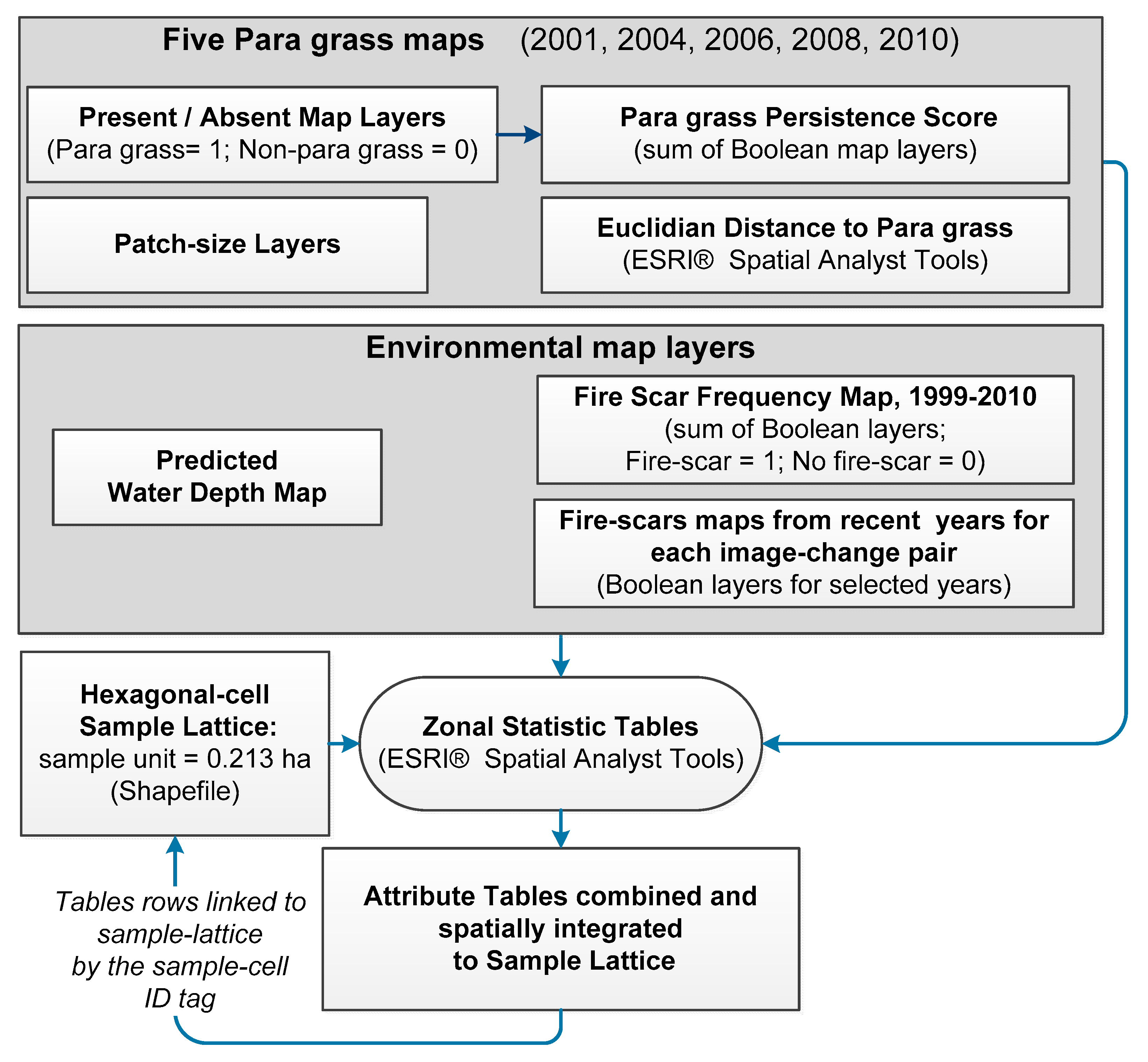
| Group | Variable | Description | Derivation |
|---|---|---|---|
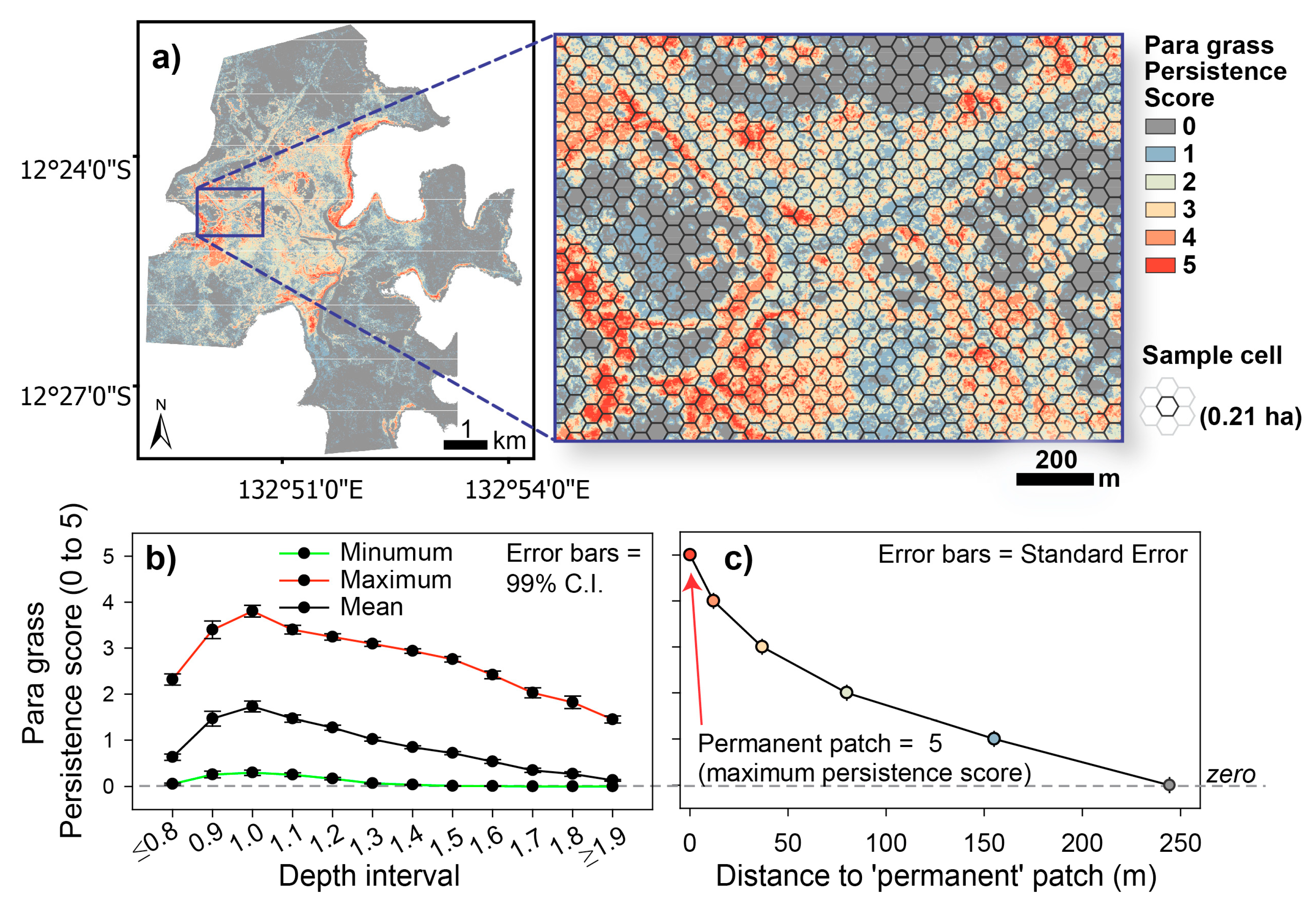
| Para Grass | Cumulative Persistence Score (CPS) | The persistence of para grass at any one location, over time (2001 to 2010). | The sum of binary map layers for para grass presence using maps 2001, 2004, 2006, 2008 and 2010 (i.e., present = 1, or not present = 0). |
| (a) Cell-density, and (b) change in cell-densities | (a) The percentage of para grass cover measured within each 0.24 ha, hexagonal, sample cell of each map layer (2001, 2004, 2006, 2008, and 2010); and (b) the negative or positive change in cell-densities, calculated for each image-difference pair in series: 2001-04, 2004-06, 2006-08 and 2008-10. | Percentage cover calculated based on the number of para grass pixels as a proportion of the total number of pixels within a hexagonal cell. Change in cover then calculated by subtraction for image-difference pair (please refer to Equations (1) and (2), below). | |
| Distance to patch and change in patch distance | The Euclidean distances (m) to nearest discrete para grass ‘patch’ over time, 2001 to 2010. Changes in patch distances were also measured for each image-pair in series: 2001-04, 2004-06, 2006-08 and 2008-10 and denoted as either an increase (+) or decrease (–) in distance. | The Euclidean distance function applied at 1 m resolution to each map. Zone statistics were then derived for each layer from the hexagonal sample matrix. Refer to Equation (3), below for the ‘change in distance’ calculation. | |
| Distance to ‘Permanent’ Patch | The Euclidean distances (m) to the nearest ‘Permanent’ patch, defined as patches with a possible maximum cumulative persistence score (CPS) of 5 | Euclidean distance function applied at 1 m resolution. The spatial analyst ‘Reclass’ function was used to generate the CPS map layer. | |
| Patch Size | Contiguous areas classified as para grass. Patch sizes (ha) were calculated for each classification layer: 2001, 2004, 2006, 2008 and 2010. | Patch areas (ha) calculated from polygon layers generated for all classifications. Georeferenced zone statistics (mean and maximum) were calculated for each respective layer using the hexagonal sample lattice. | |
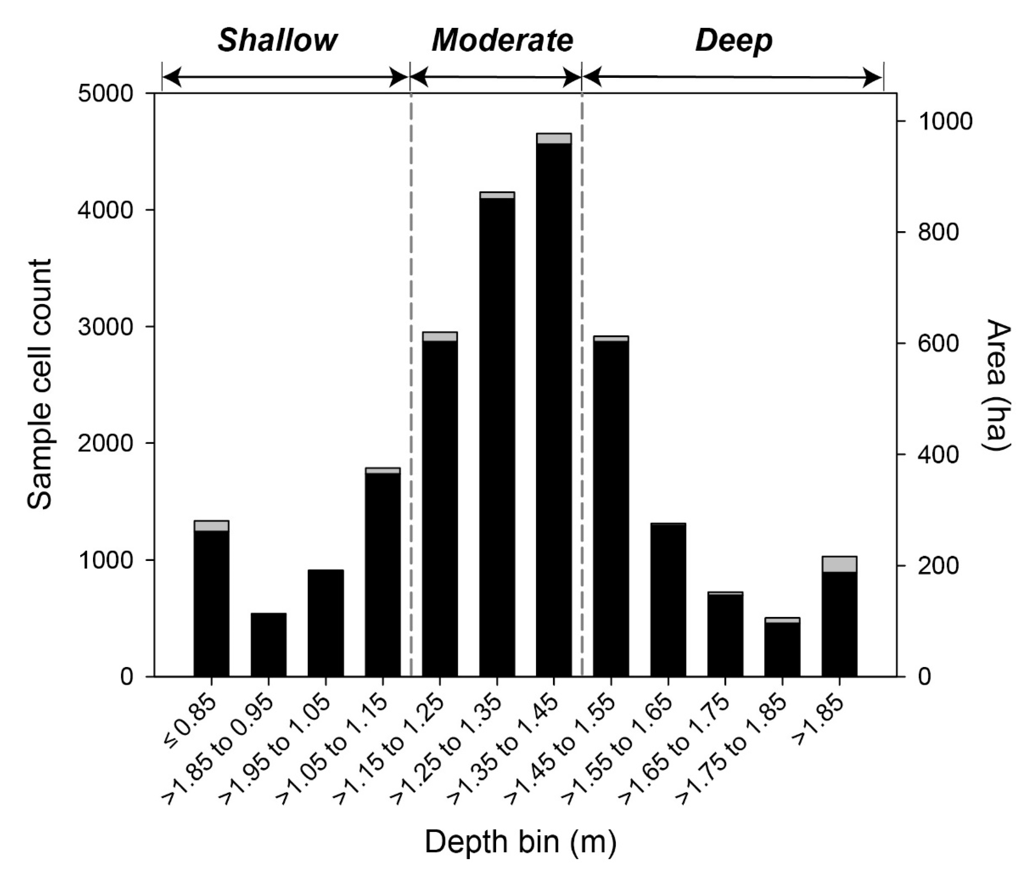
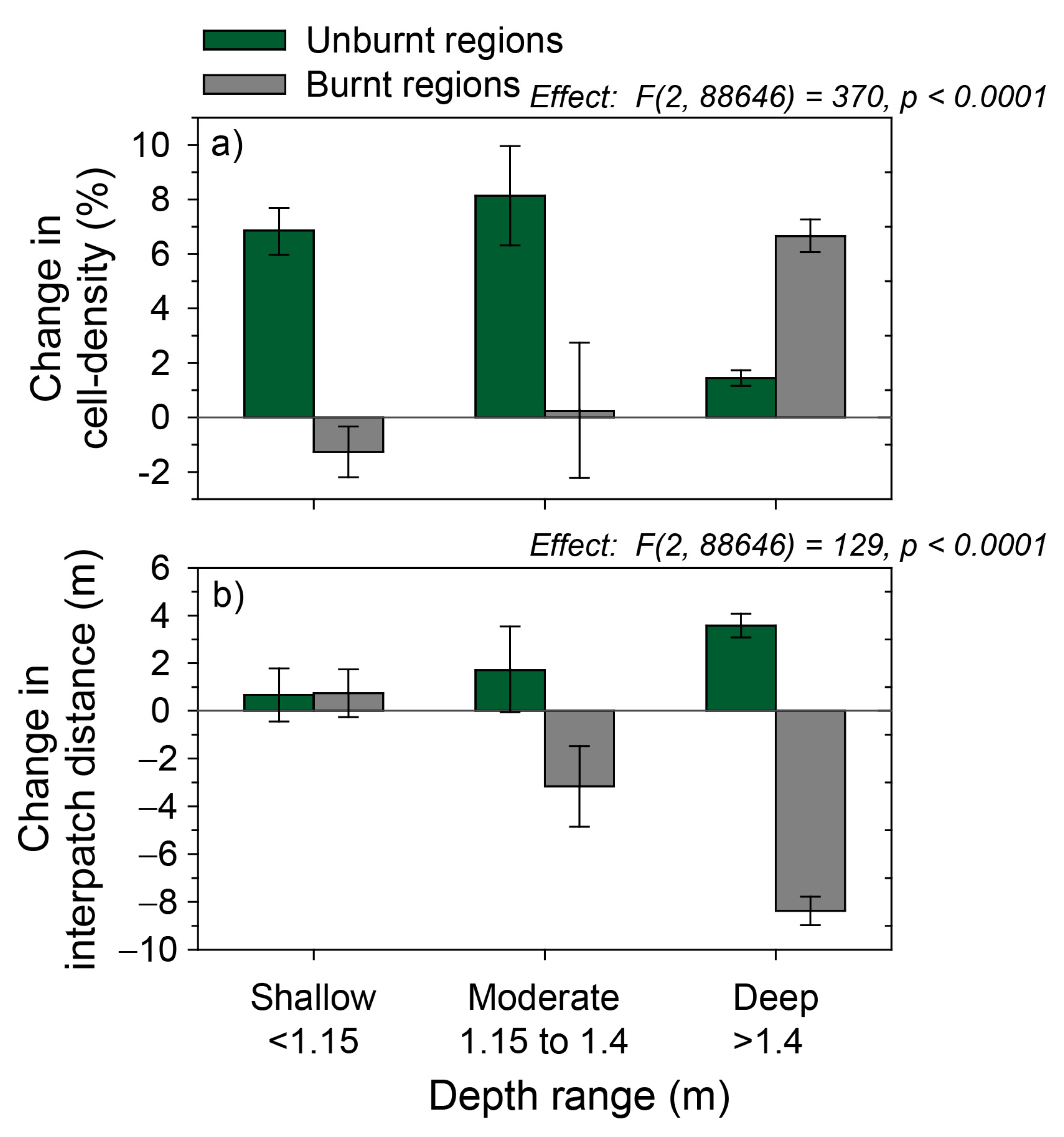
| Other | Depth habitat | Used in the analysis of variance (ANOVA) of para grass change in relation to three depth categories: ‘Shallow’, ‘Moderate’ and ‘Deep’. Selection of the depth ranges of each depth category were based on the distribution of para grass in relation mapped depth [51}. | |
| Previous dry-season fire | The burnt (or unburnt) areas mapped in the first dry-season period between each image- difference pair (i.e., 2001-04, 2004-06, 2006-08 and 2008-10.) | The fire-scar maps derived from Landsat representing years 2003, 2005, 2007 and 2009 [51]. |
| Class | Number of Pixels | Accuracy | Kappa Statistic | Error Rate (%) | |||||||
|---|---|---|---|---|---|---|---|---|---|---|---|
| Image | Reference | Classified | Correct | Producers | Users | Overall | Producers | Users | Overall | Omission | Commission |
| IKONOS (2001) | 410897 | 413727 | 377619 | 92 | 91 | 96 | 0.90 | 0.89 | 0.89 | 8 | 9 |
| QuickBird (2004) | 707180 | 756735 | 664166 | 94 | 88 | 96 | 0.92 | 0.84 | 0.88 | 6 | 12 |
| QuickBird (2006) | 617425 | 643414 | 590333 | 96 | 92 | 96 | 0.94 | 0.88 | 0.91 | 4 | 8 |
| QuickBird (2008) | 625118 | 700247 | 618718 | 99 | 88 | 97 | 0.99 | 0.88 | 0.91 | 1 | 12 |
| WorldView (2010, R1*) | 86461 | 89831 | 74124 | 86 | 83 | 99 | 0.85 | 0.82 | 0.83 | 14 | 17 |
| WorldView (2010, R2*) | 273762 | 279851 | 264567 | 96.6 | 95 | 97.6 | 0.95 | 0.93 | 0.94 | 3.4 | 5 |
| Cover Measurement | Depth Range (m) | Linear Regression Results | ||||
|---|---|---|---|---|---|---|
| Slope (b) | R | Adjusted R2 | p | Sig. | ||
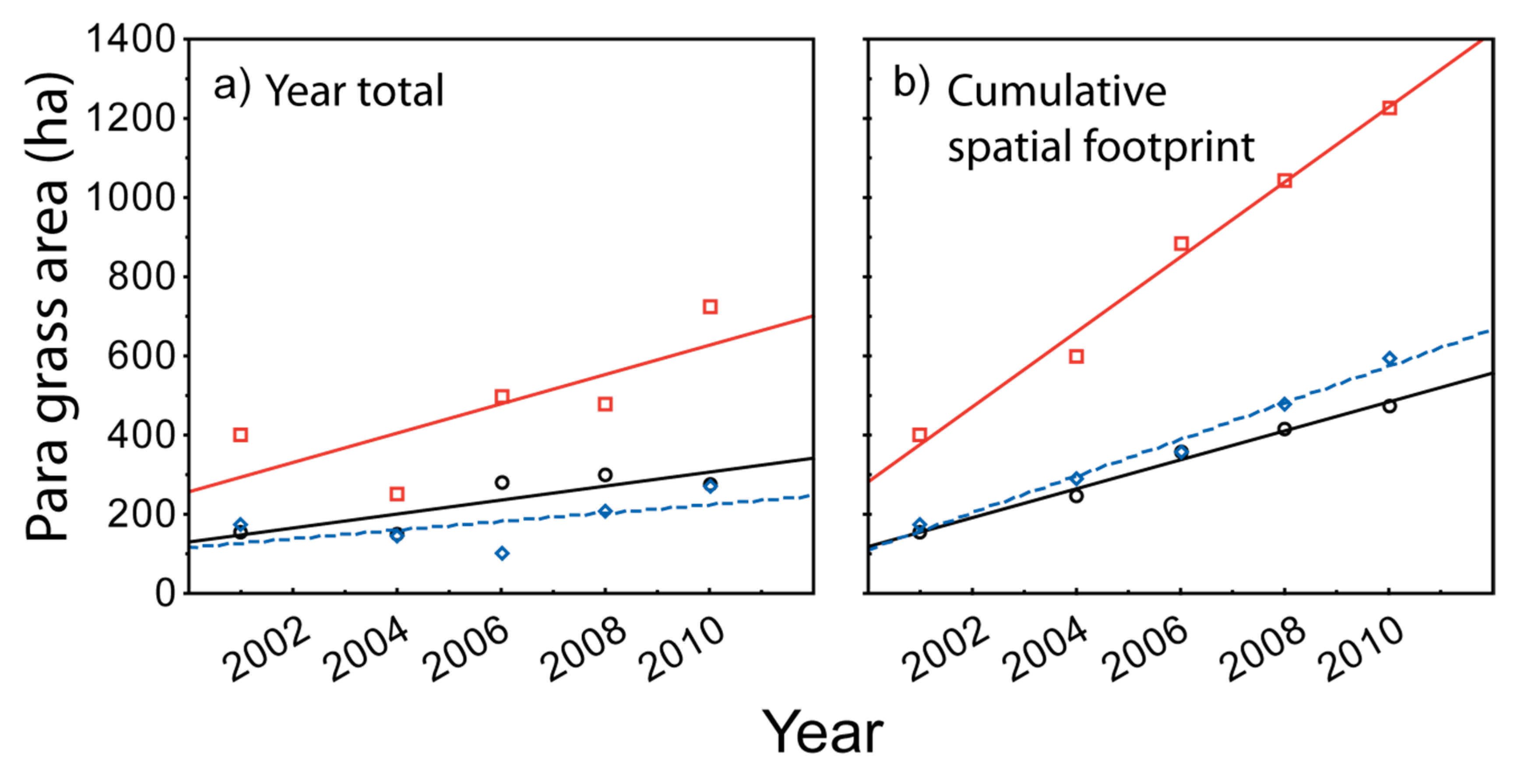
| Year by year totals | Shallow  ≤ 1.15 m ≤ 1.15 m | 18 | 0.84 | 0.61 | 0.074 | * |
Moderate > 1.15 to 1.4 > 1.15 to 1.4 | 37 | 0.75 | 0.42 | 0.141 | * | |
Deep > 1.4 > 1.4 | 11 | 0.59 | 0.13 | 0.297 | ns | |
| Cumulative ‘footprint’ overtime | Shallow  ≤ 1.15 m ≤ 1.15 m | 37 | 0.99 | 0.98 | 0.001 | *** |
Moderate > 1.15 to 1.4 > 1.15 to 1.4 | 95 | 0.99 | 0.98 | 0.001 | *** | |
Deep > 1.4 > 1.4 | 46 | 0.99 | 0.98 | 0.001 | *** | |
© 2019 by the authors. Licensee MDPI, Basel, Switzerland. This article is an open access article distributed under the terms and conditions of the Creative Commons Attribution (CC BY) license (http://creativecommons.org/licenses/by/4.0/).
Share and Cite
Boyden, J.; Wurm, P.; Joyce, K.E.; Boggs, G. Spatial Dynamics of Invasive Para Grass on a Monsoonal Floodplain, Kakadu National Park, Northern Australia. Remote Sens. 2019, 11, 2090. https://doi.org/10.3390/rs11182090
Boyden J, Wurm P, Joyce KE, Boggs G. Spatial Dynamics of Invasive Para Grass on a Monsoonal Floodplain, Kakadu National Park, Northern Australia. Remote Sensing. 2019; 11(18):2090. https://doi.org/10.3390/rs11182090
Chicago/Turabian StyleBoyden, James, Penelope Wurm, Karen E. Joyce, and Guy Boggs. 2019. "Spatial Dynamics of Invasive Para Grass on a Monsoonal Floodplain, Kakadu National Park, Northern Australia" Remote Sensing 11, no. 18: 2090. https://doi.org/10.3390/rs11182090
APA StyleBoyden, J., Wurm, P., Joyce, K. E., & Boggs, G. (2019). Spatial Dynamics of Invasive Para Grass on a Monsoonal Floodplain, Kakadu National Park, Northern Australia. Remote Sensing, 11(18), 2090. https://doi.org/10.3390/rs11182090